Generalized Linear Models.md

Overview

After attending some lectures and reviewing several materials, it took me a considerable amount of time to grasp the basics of the exponential family and understand why and how they can be applied to GLMs (Generalized Linear Models). The fundamentals of GLMs will be thoroughly explained in this article.

We will begin with exponential families, then cover the basics of some machine learning algorithms (e.g. linear regression and logistic regression) and discover what they have in common. In the end, we will integrate all these concepts to derive a larger scale of models and to understand the reasons behind these desirable properties.

Note: This article is aimed at providing an overview, and some mathematical details are omitted. Readers can complete proofs on their own or by checking the material listed at the end of the article.

Exponential Family

The exponential familiy involves a set of probability distributions whose probability density function can be expressed as

Or in canonical form

Where is the natural parameter or the canonical parameter, is the sufficient statistic, and is the log partition function which normalizes the densities.

Properties

Property 1:

Property 2:

Property 3: Let be the log-likelihood function, then

Property 4: is concave.

Linear Regression and Logisitic Regression

Now, let's review two of the most important algorithms in the field of machine learning: (ordinary) linear regression and logistic regression.

Linear Regression

Suppose we have samples and features. Let be the input vector and the target of the -th sample respectively. We would like to find the parameters that best fits the linear relationship between features and targets.

A common choice is to use normal distribution as the probabilistic assumption. Here we assume for the -th sample, so the likelihood function is given by

Take the derivatives of the log-likelihood and we will get

Let be the model prediction given input , we have

So the update rule with gradient ascent is given by

Where is the learning rate.

This update rule is computationally efficient and makes intuitive sense. Consider the following cases: - Case 1: The prediction is smaller than the target. Increase the parameter if the corresponding feature is positive, and vice versa. - Case 2: The prediction is larger than the target. Decrease the parameter if the corresponding feature is positive, and vice versa. - Case 3: The prediction is equal to the target. In this case, no update is required.

Logistic Regression

Consider the classic binary classification problem, where the target variable can be either or .

A common choice is to use the Bernoulli distribution as the probabilistic assumption. Here we assume as the mean of the Bernoulli distribution (which is also ). So the likelihood function is given by

where is the logistic function:

By taking the derivatives of the log-likelihood, we can get almost the same update rule as linear regression. Let , then we have

To derive a larger scale of models with the elegant update rule , we will introduce the generalized linear models.

Generalized Linear Models

Overdispersed Exponential Family

Overdispersed exponential family is a generalization of exponential family, with a dispersion parameter involved. The probability density function can be expressed as:

Similar to the exponential family, it has the following properties:

Property 1:

Property 2:

Property 3: , where .

Property 4: is concave.

Note that these properties still hold no matter whether the probability distribution is continuous or discrete.

From my point of view, though overdispersed exponential familiy is more flexible compared to the ordinary exponential family as it involves the dispersion parameter , often plays no significant role when it comes to optimize model parameters – And that's the reason why I set in the derivation of the update rule in ordinary linear regression. If you regard as a parameter of the probability distribution but not a constant, you will get almost the same result.

Introduction to GLMs

We begin with the linear predictor . Here, denotes the model parameters and denotes a sample of the dataset.

Then, we need probabilistic assumpsions about the conditional probability of the target given for GLMs, which should be in the overdispersed exponential familiy: Let , then we have 。

And how do we connect with ? We can use link functions, which maps the mean to the linear predictor . When always holds, we can refer to the link function as canonical link function。

Because using a canonical link function is a common choice(though counterexamples do exist), we will only focus on models using canonical link functions.

The figure below shows the relationships between and (from stackexchange):

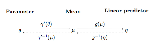
Note that in the figure is the same as in this article.

So what is the task of the model? It should compute the linear predictor based on . When the link function is canonical, is the same as , so it will predict as .

It can be proved that the update rule for any generalized linear model using gradient ascent is always the following:

Linear Regression

As I mentioned above, the probabilistic assumption is the normal distribution, which is in the overdispersed exponential family:

As , we have

Conclusion: For a generalized linear model with normal distribution as the probabilistic assumption, ordinary linear regression model with should be used.

Logistic Regression

In binary classification tasks, the probabilistic assumption is the Bernoulli distribution, which is also in the overdispersed exponential family:

Let , we have

Take the derivative of and we will get

Which is the logistic function.

Conclusion: For a generalized linear model with Bernoulli distribution as the probabilistic assumption, logistic regression model with should be used.